Beer Game
How do I play the Opex Analytics Beer Game?
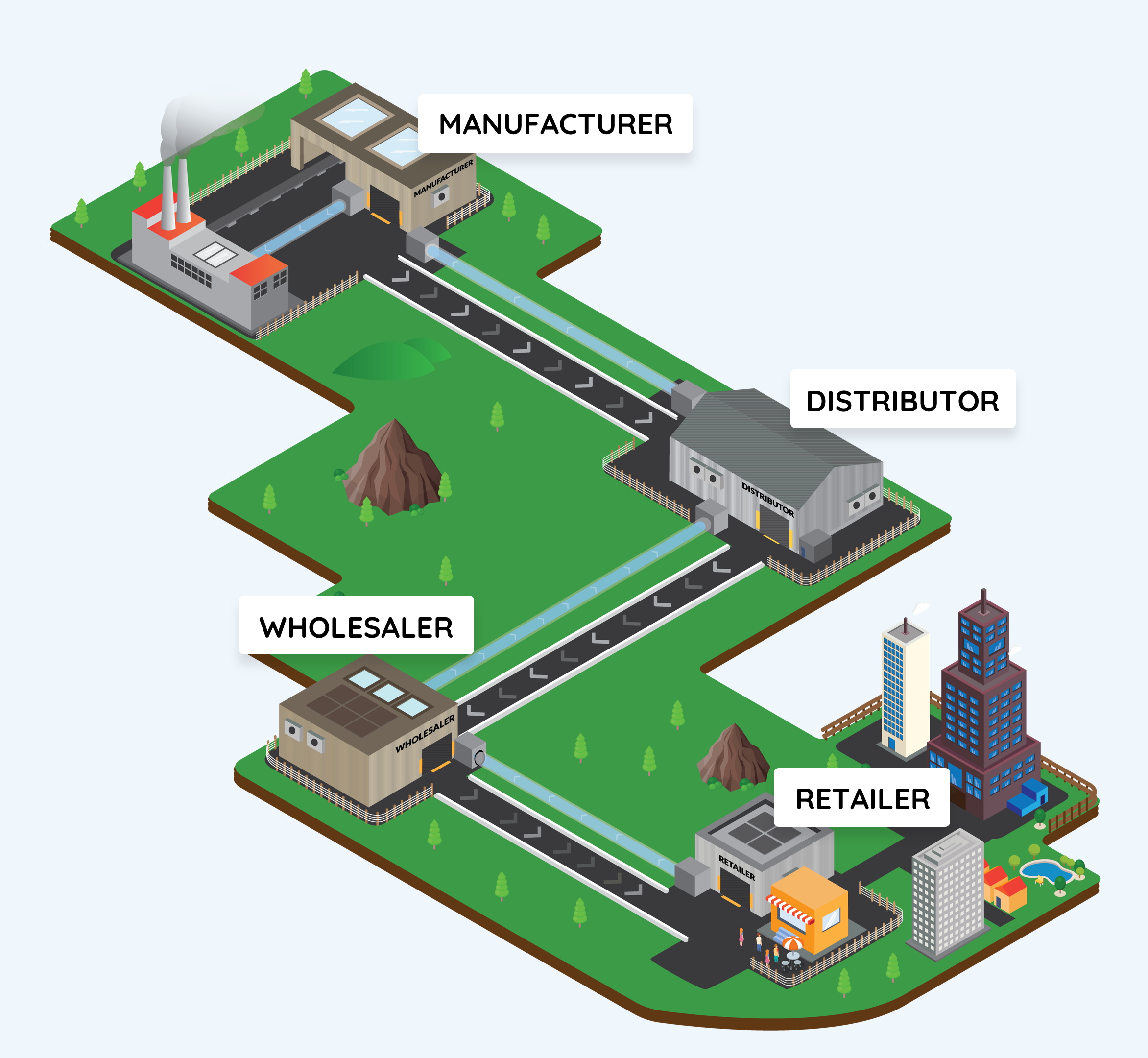
The game begins by placing you within an existing supply chain. In any given
period, the Retailer receives demand for cases of beer from a customer; these
demands are generated by the game. The Retailer then places orders for beer
from the Wholesaler, who orders from the Distributor, who orders from the
Manufacturer. Each of these stages, in turn, fills as much of the incoming
order as it can from its on-hand inventory. Any additional demand is
backordered, which means it is filled in a future period as inventory becomes
available.
You pay a cost for on-hand inventory (inventory left in your facility), as well
as for unmet demand (backorders) at the end of each period. (See Game Settings
below.) Your ultimate goal is to keep the total cost for your supply chain
team—including all players throughout all time periods—as small as possible.
Inventory Level (IL) Defined
A key metric to keep your eye on is your inventory level (IL), which equals your on-hand
inventory minus your backorders. It can be positive, negative, or zero at any time. Let’s
assume you are playing the role of the Wholesaler. You start a period with 5 cases of beer
on hand (so IL = 5). You receive an order from the Retailer for 8 cases, and you receive a
shipment from the Distributor containing 6 cases. At the end of the period, your IL = 5 − 8
+ 6 = 3 cases.
In the next period, you begin with IL = 3. Suppose you receive an order from the Retailer
for 10 cases and a shipment from the Distributor with 5 cases. Your ending IL = 3 − 10 + 5
= −2 cases. These “negative cases” of beer are really backorders—cases that you “owe” to
your customer.
In other words, whenever IL > 0, you have inventory on hand (equal to IL cases), and
whenever IL < 0, you have backorders (equal to −IL cases).
Getting Started: Game Settings
In what follows, we will describe the parameters under the Classic (our
default) setting of the game as well as the additional options you may choose
for each setting. Note that these predefined parameter settings are available
through the “Change Settings” button on the Default Settings page, which allows
you to change any of the pre-defined parameters to whatever values you like.
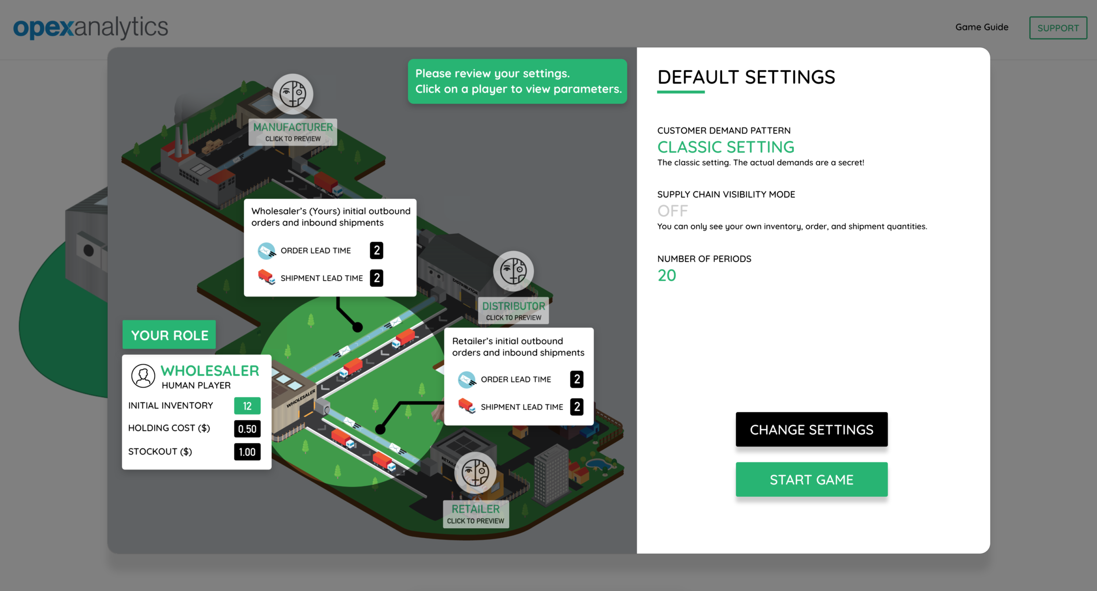
The default settings are as follows:
- You play as the Wholesaler
- You have no AI teammates
- All of your teammates are played by “Human-Like” computerized players, which means their ordering patterns mimic how humans tend to play the game
- All of your teammates are played by “Human-Like” computerized players, which means their ordering patterns mimic how humans tend to play the game
- Customer demands follow the pattern used in the classic version of the game. (The actual demands are a secret until you play the game)
- Order and shipment lead times are 2 periods each, for every player except the Manufacturer, who instead has an order lead time of 1 period
- For every player, holding costs are $0.50 per case on hand and stockout costs are $1.00 per case backordered
- Supply chain visibility mode is off, which means that you can only see your own inventory levels and outbound order and shipment quantities
- The game will last for 20 time periods
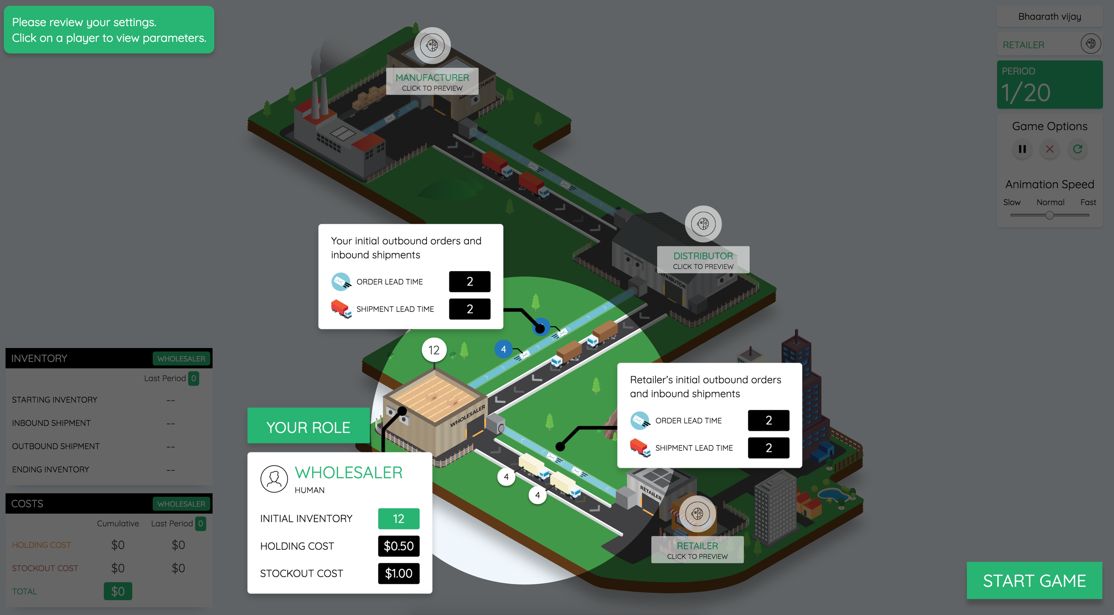
These settings are displayed on the Default Settings page. You can click on the
other players to view their settings:
If you are satisfied with the default settings, click Play Game. Otherwise,
click Change Settings. Next, we’ll walk through the options you have within the
Change Settings screen.
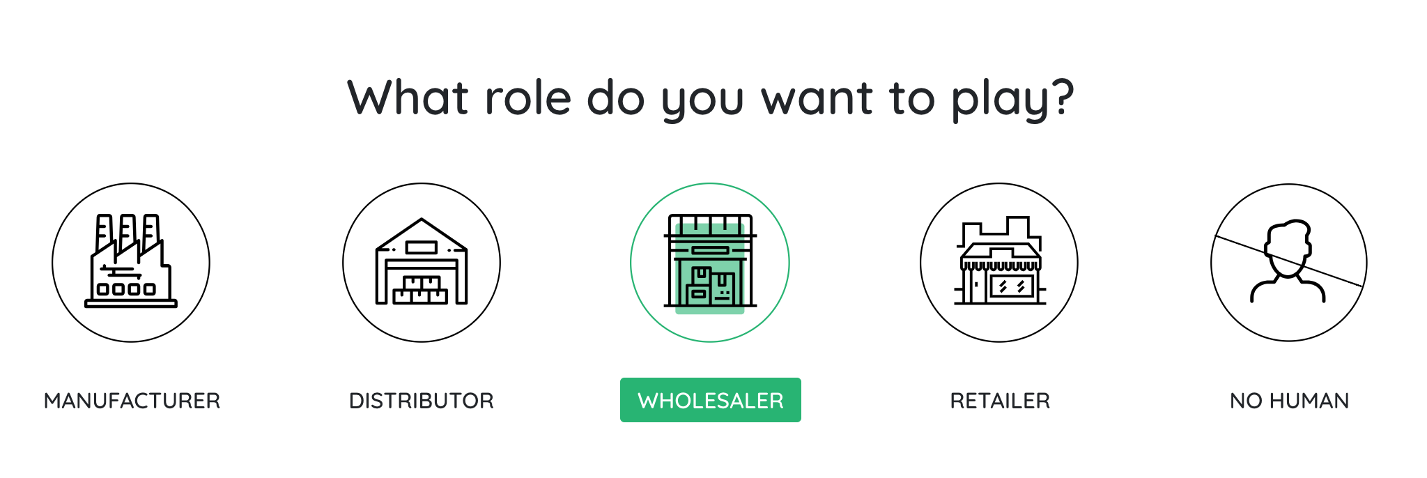
First, you can choose which role you would like to play. By default (as
discussed above), you play the Wholesaler, but you can change this to any of
the other three supply chain nodes. Or, you can also choose not to play at all.
In this case the team will consist of four computerized players, with no human
in the loop.
Once you have chosen your own role and the AI’s role (if any), you can choose
how you want the remaining, computerized, players to play.
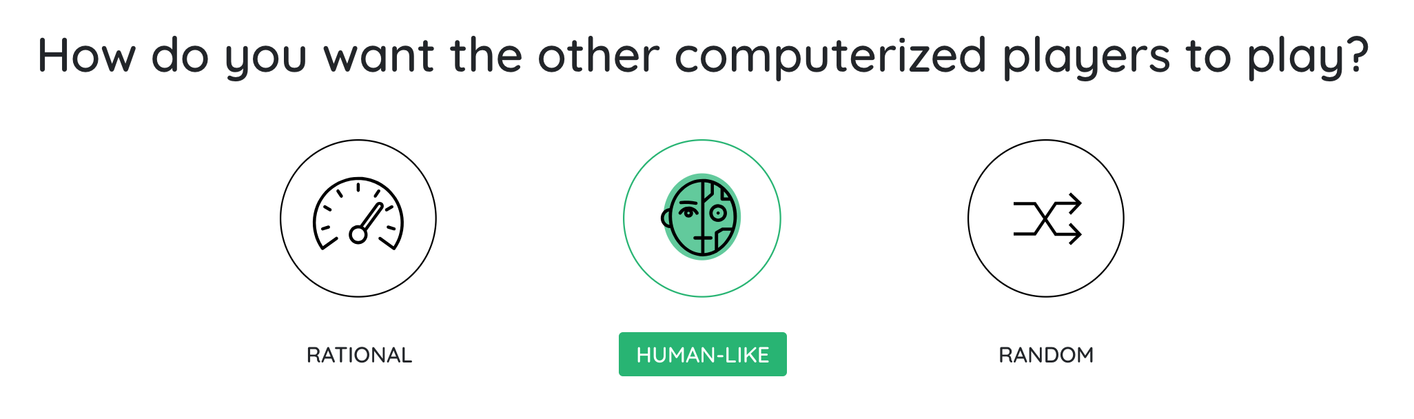
The options for the computerized players are as follows:
- Human-Like (default): The player uses the “anchoring and adjustment” formula by Sterman (1989), which is meant to emulate how humans play the beer game. The player tends to over-react when the inventory level and pipeline inventory are low or high.
- Rational: The player follows a base-stock policy.strong> That means that in each period, the player places an order to bring its inventory position (equal to its inventory level plus any units that have been ordered but not yet received) equal to a fixed number called the base-stock level. Equivalently, in each period (except the first), the player places an order equal to the size of the demand that it received.
- Random: The player chooses order quantities randomly, within a particular range.
Next, you can choose the demand pattern that the Retailer’s customers will
follow.
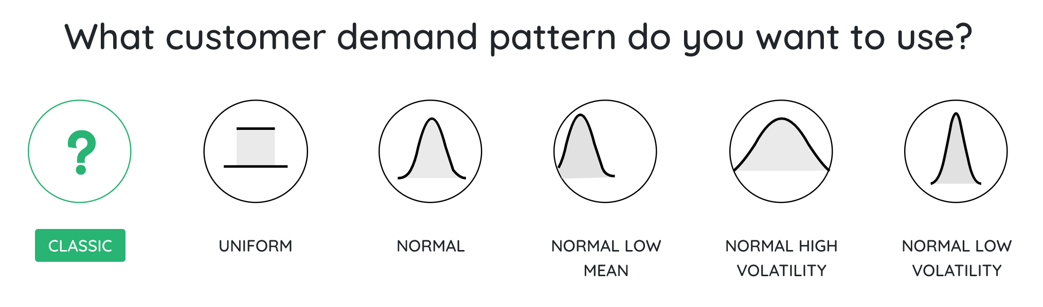
The options are:
- Classic (default): This is the classic setting of the original beer game, from the famous paper by Sterman (1989). The actual demands are a secret. (You’ll find out at the end of the game.)
- Uniform: The demands come from a uniform probability distribution on the integers 0, 1, …, 8. That is, the demands can be 0, 1, …, or 8 with equal probability.
- Normal: The demands come from a normal probability distribution with a mean of 50 and a standard deviation of 20. This setting comes from the paper by Chen and Samroengraja (2000).
- Normal, Low Mean: The demands come from a normal probability distribution with a mean of 10 and a standard deviation of 2.
- Normal, High Volatility: The demands come from a normal probability distribution with a mean of 10 and a standard deviation of 30.
- Normal, Low Volatility: The demands come from a normal probability distribution with a mean of 10 and a standard deviation of 5.
Note: Our AI agent is only trained to play under some of the
demand patterns. Therefore, if you have chosen to have an AI agent on your
team, some of the demand patterns will be disabled.
The last settings screen contains a number of options:
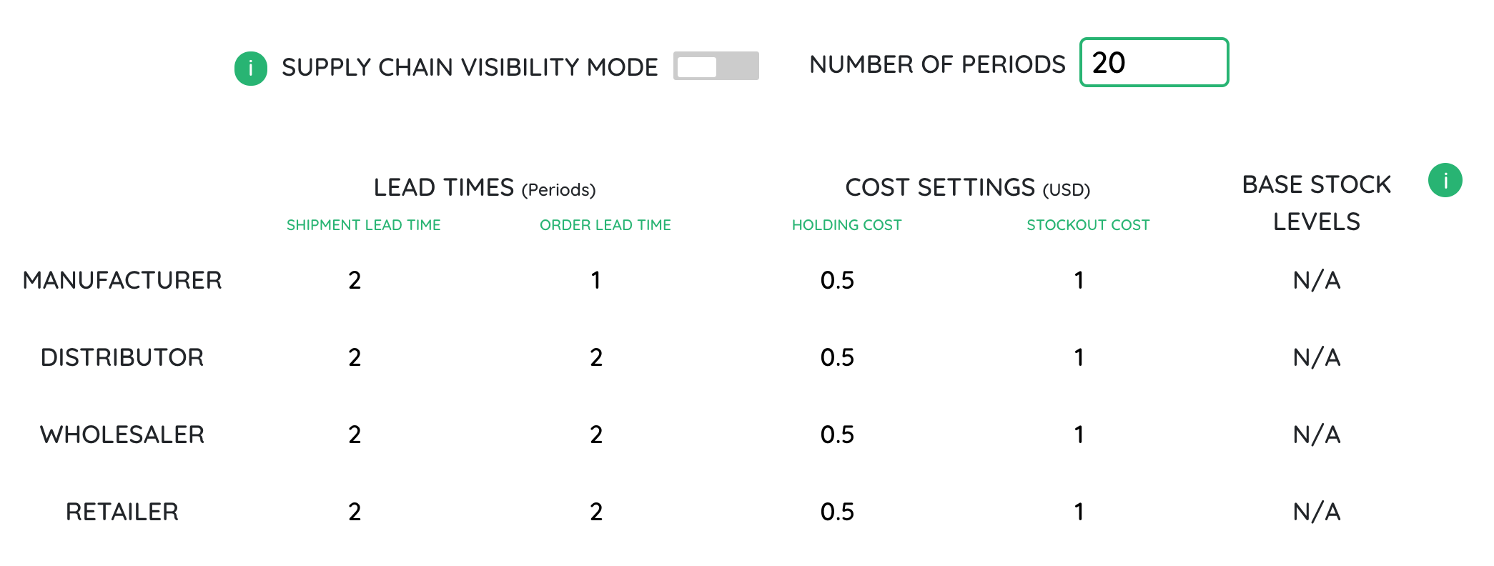
Let’s start with the
Lead Times. When you place an order to
your supplier (i.e., your upstream partner), you don’t receive that beer right
away. In fact, your supplier doesn’t even receive your order right away.
Instead, your supplier receives your order after a 2-period (by default)
order lead time.* In addition, once your supplier ships beer
to you, you receive it after a 2-period (by default)
shipment lead time.
Considering all this, bear in mind that you won’t receive each order you place
for at least 4 periods. Why “at least”? Because your supplier might be out of
stock, in which case you’ll also have to wait until your supplier’s stock is
replenished, in addition to the usual 4 periods of order and shipment lead
time.
*The Manufacturer has only a 1-period order lead time.
Now let’s move on to the Cost Settings. The default holding and stockout costs
are as follows:
- For the Classic and Uniform demand patterns, the holding cost is $0.50 per case and the stockout cost is $1.00 per case.
- For the Normal demand patterns, the holding cost is $1.00 at the Retailer, $0.75 at the Wholesaler, $0.50 at the Distributor, and $0.25 at the Manufacturer. The stockout cost is $10.00 at the Retailer. The other stages have no stockout cost.
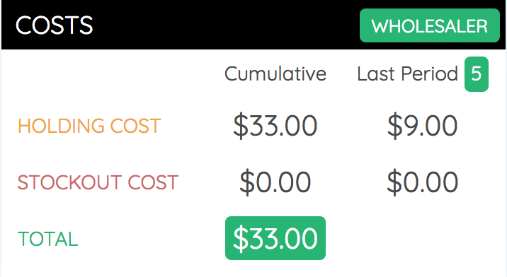
Remember that you pay the holding cost when your inventory level (IL) is
positive, and you pay the stockout cost when your IL is negative. In every
period, your ending inventory level is calculated as IL = [starting IL] −
[order received] + [shipment received].
The
Base-Stock Levels only apply to computerized players that
are set to Rational mode. A Rational player follows a base-stock policy, which
means in every period its order quantity is calculated to bring its inventory
position (equal to the IL plus the items that it has ordered from its supplier
but has not yet received) equal to the base-stock level.
Finally, you can choose the
Number of Periods that the game
should last, and you can turn Supply Chain Visibility Mode on or off. When
Supply Chain Visibility Mode is off, you can see the
quantities of the orders and shipments that you send, but not any of your
teammates’ orders or shipments anywhere else in the supply chain. This is the
typical setting for the beer game. When Supply Chain Visibility Mode is on, you
can see all of these values.
After selecting your settings you will click Start Game and see a preview of
your global settings, as well as the option to view the other players’ settings
prior to kicking off the game play.
Playing the Game
In each period of the game, the following events will occur, in this order:
- You learn your inbound order quantity:
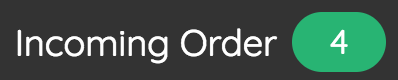 If you are the Retailer, this is the customer demand; otherwise, it is the order placed by your downstream teammate, who sent it 2 periods ago (assuming that your downstream teammate’s order lead time is 2).
 - You then choose your outbound order quantity:
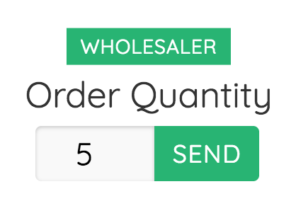 This is your only decision in each time period. Once you place your order, it heads upstream in an order envelope. It will arrive at your upstream teammate after 2 periods (assuming that your order lead time is 2).
 - Next, you receive your inbound shipment from your upstream teammate, who sent it 2 periods ago (assuming your upstream teammate’s shipment lead time is 2 periods). (If you are the Manufacturer, then your “upstream teammate” is your manufacturing process. It always ships whatever you order.)
- Finally, you send your outbound shipment. If you are any player other than the Retailer, your shipment heads downstream in a truck and arrives at your downstream teammate after 2 periods (assuming your downstream teammate’s shipment lead time is 2). If you are the Retailer, then your outbound shipment is just the items that you provide to the customer.
- Holding and stockout costs are applied to your ending inventory level:
Notice that between steps 2 and 3, your supplier sends orders to his or her
supplier, and so on up the supply chain, all the way to the Manufacturer. The
Manufacturer then turns around and ships beer to the Distributor, and so on down
the supply chain until it reaches you and then ultimately the customer.
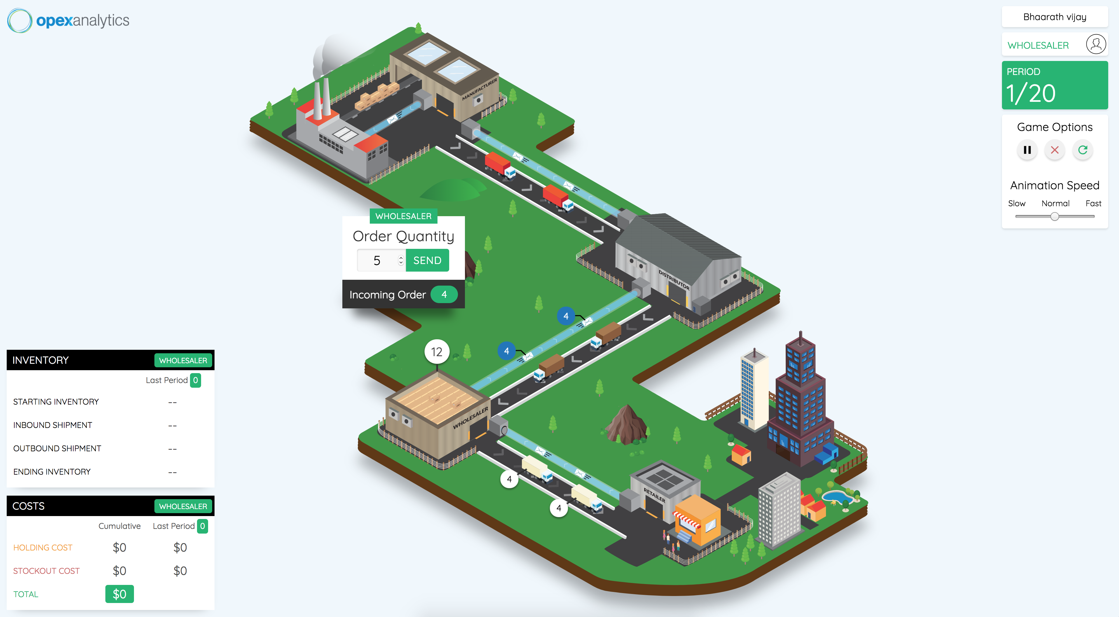
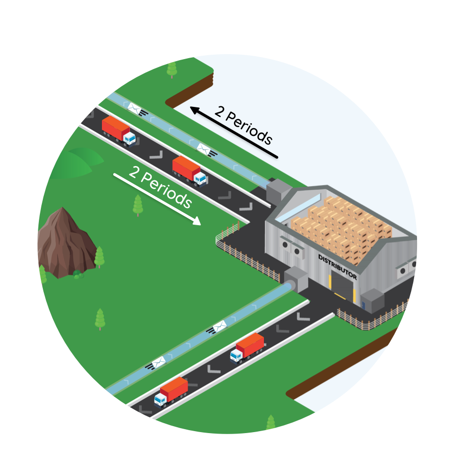
In the Opex Analytics Beer Game, orders are depicted as envelopes traveling
upstream along an “information pipeline,” and shipments are depicted as trucks
traveling downstream along a road.
When the game starts, each player already has some items on hand in inventory, as
well as some pending outbound orders (in the envelopes traveling upstream from the
player) and some pending inbound shipments (in the trucks traveling downstream to
the player). You can think of the game as starting with a supply chain that is
already in progress.
During the game, you’ll see your changing inventory level in a bubble above your
facility. Remember that negative inventory levels mean backorders. The number of
boxes in your facility will also give you a visual cue as to how small or large
your inventory level is as well. Red boxes represent backorders.
The game ends after a fixed number of periods, specified in the Game Settings page.
Game Results
After the game ends, you’ll get a summary of your results and a comparison of your
performance with that of our computerized players:
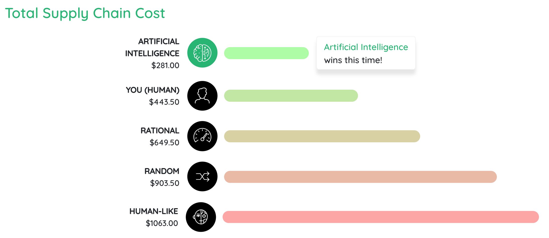
Our computerized agents played the same game you did, in the same role, with the
same settings and demands. In this case, you (the human) played as the Wholesaler
and had a cost of $443.50. Our AI agent beat you, with a score of $281. Our
Rational, Random, and Human-Like players did worse than you.
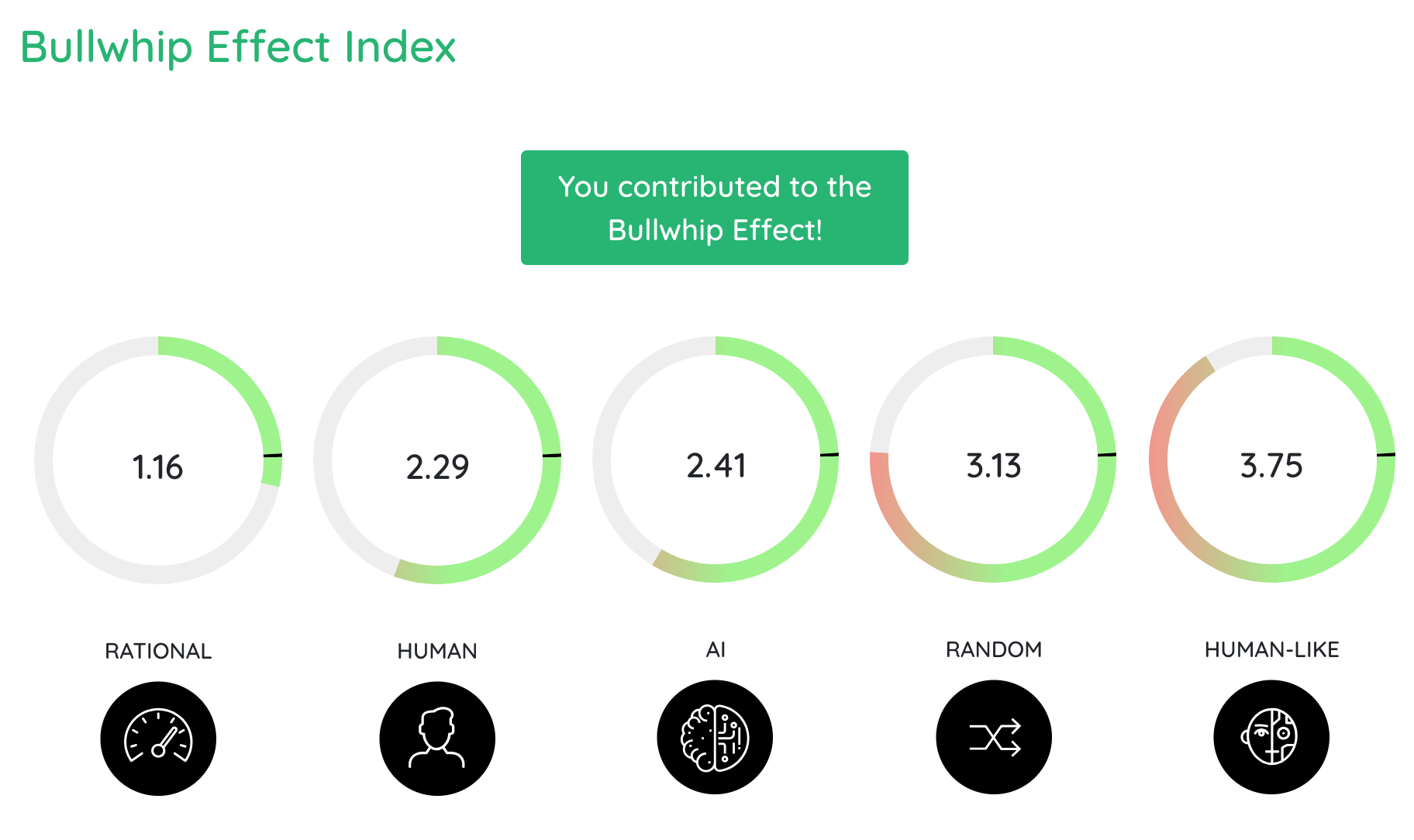
The second game summary report provides you with a comparison of your “Bullwhip
Effect Index”:
The bullwhip effect index (BEI) is the variance of your order quantity divided by
the variance of the order quantity you received from your downstream partner (or
the customer demand):
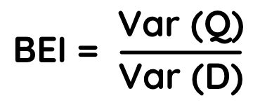
where Q is the list of your order quantities and D is the list of your demands.
When people play the beer game, they often start to panic when their inventory
level gets low or negative, leading them to place large orders—even if there is
plenty of inventory on its way, in the pipeline. Later, when those huge orders
arrive, the inventory levels get too large, so the player panics and starts placing
tiny orders—even if the pipeline inventory is insufficient to meet the upcoming
demands. This panicky behavior is undesirable, and it leads to the bullwhip effect.
Players who can avoid panicking and stay calm will produce less bullwhip effect,
which will often lead to smaller costs.
In essence, the BEI is a measure of the “level of panic” or “level of calm” you
brought to the supply chain
- If BEI > 1, then your orders are more volatile than your customer’s orders, so you are contributing to the bullwhip effect. This is the “level of panic” you contributed.
- If BEI < 1, then your orders are less volatile than your customer’s orders, so you are reducing the bullwhip effect. This is the “level of calm” you contributed.
- If BEI = 1, then you are keeping your cool, i.e., keeping the order volatility stable. This means you stayed in step with your teammates, neither panicking nor adding calm to the ordering patterns.
In the picture above, you had a BEI of 2.29, so you made the bullwhip effect worse
by adding to the panic.
It is natural to assume that you should aim for a BEI of 0. However, this is not at
all true. Instead, “good” BEIs tend to be close to 1. What you must remember is
that while reducing the bullwhip effect is good, it is not the only factor. To take
an extreme example, if you order 0 in every period, your BEI = 0, but this is a
terrible policy! In general, it’s good to have a smaller BEI, as long as you can do
so without sacrificing good inventory management, that is, without forcing your
costs to increase.
If you are interested in looking into the overall supply chain performance even
further, you can also get period-by-period graphs of your team’s performance using
the additional “Reports” shown in the bottom section of the Game Reports screen.
These provide views of the inventory level, cumulative cost, order quantity, fill
rate, and BEI, for each of the four players on your team and in total:
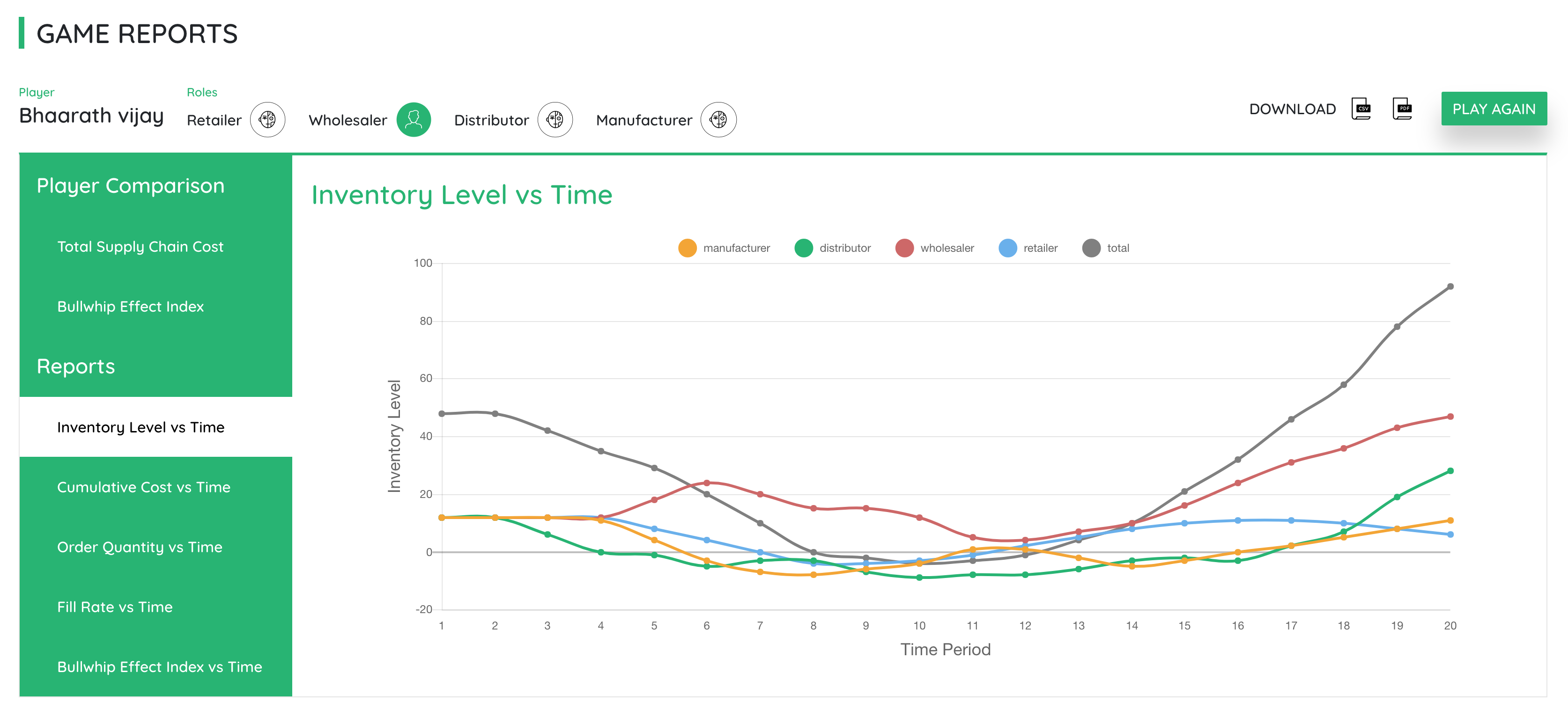
Note that you can also turn a data series on and off by clicking on its associated
listing within the graph legend.
All reports can be downloaded as either a comma-separated value (CSV) file or a PDF
file using the links at the top right of the page.